Georg Nees, Processing, and a Schotter Tutorial

By Jim Plaxco

Georg Nees was one of the pioneers of computer art. Born in Germany in 1926, he was a pupil of Max Bense, the founder of Information Aesthetics. It is believed that Nees' solo show at the University of Stuttgart in February 1965 was the first exhibition of computer art. One of Georg Nees' signature pieces is Schotter (Gravel in German), a plotter drawing created circa 1965. It was this piece that inspired me to create my own series of Cubic Disarray algorithmic art works. The pieces in this collection are:

• Cubic Disarray: Division
• Cubic Disarray: Bisection
• Cubic Disarray: Impending Unity
• Cubic Disarray: Point of Radiance
• Cubic Disarray: Turbulence

These are all works that I've only now decided to add to my web site. It was this decision that led me to attempt to reproduce Nees' original Schotter and to turn that effort into a tutorial. For this recreation I am using Processing. Processing is an open source programming language with its own IDE (Integrated Development Environment) created for practitioners of the new media arts. If you want to experiment with the program that follows you will need to download and install Processing. Processing is free and is available for multiple platforms. Visit http://processing.org/ for more information and to download Processing for your computer.

In the original Schotter, Nees creates a grid of squares 12 across by 22 down. As the drawing of the squares progresses from top to bottom, the amount of disorder increases. This disorder takes two forms. First is in the positioning of each square, second is in its rotation. Images of the original Schotter and the Processing recreation are shown below.

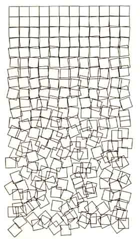Original Schotter by Georg Nees.

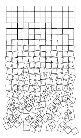Processing version of Schotter.

Source Code for the Recreation of Georg Nees' Schotter

Before proceeding with the tutorial, take the time to look over the following source code. Alternatively, you can download the Nees_Schotter.pde source code file to your computer and edit the file as the tutorial proceeds.

// Georg Nees Schotter Reproduction by Jim Plaxco, www.artsnova.com
int columns = 12;       // number of columns of squares
int rows = 22;          // number of rows of squares
int sqrsize=30;         // size of each square
float rndStep=.22;      // Rotation Increment in degrees 
float randsum=0;        // Cumulative rotation value 
int padding=2*sqrsize;  // margin area
float randval;          // random value for translation and rotation
float dampen=0.45;      // soften random effect for translation
 
void setup() { 
  size((columns+4)*sqrsize,(rows+4)*sqrsize); 
  background(255);   // set background color to white
  stroke(0);         // set pen color to black
  smooth();          // use line smoothing 
  noFill();          // do not fill the squares with color
  rectMode(CENTER);  // use x,y value as the center of the square
  noLoop();          // execute draw() just one time
} // end of setup()
 
void draw() {
  for (int y=1; y <= rows; y++){
    randsum += (y*rndStep);  // Increment the random value
    for (int x=1; x <= columns; x++) {
      pushMatrix();
      randval = random(-randsum,randsum);
      translate( padding + (x * sqrsize) - (.5*sqrsize) + (randval*dampen),
		     padding + (y * sqrsize) - (.5*sqrsize) + (randval*dampen));
      rotate(radians(randval));
      rect(0,0,sqrsize,sqrsize);
      popMatrix();
    } // end of x loop
  } // end of y loop
} // end of draw()

Variables: Thinking about the problem to be solved, I identified the variables shown in lines 2 - 9 as being necessary to implement a solution. In programming, I always prefer using variables as opposed to values because variables facilitate experimentation. For example, you will note that the screen to which the program draws is sized based on the values of the variables associated with the size of each square, the number of rows of squares, and the number of columns of squares (see line 12).

setup() Function: The setup() function (lines 11-19) is called once in order to perform initialization. The only noteworthy statement in setup() is line 12 where the variables columns, rows, and sqrsize are used to determine the size of the canvas or window.

draw() Function: The draw() function (lines 21-34) is where the actual computation and drawing takes place. The draw() function will be executed only once because of the noloop() statement in line 18. Two loops are used to control the drawing's progress. The outer loop (line 22) is responsible for stepping through the rows of squares one at a time with y being used to indicate the current row number. Each time this loop is executed, the cumulative value of the random factor randsum is incremented (line 23). In other words, the size of the random factor that controls how the squares are drawn increases as we proceed from the first row to the last row.

The inner loop (line 24) is responsible for stepping through the column of squares in each row with x being used to indicate the current column. It is in this loop that the screen coordinates are translated (moved) for each square and a rotation applied to each square. The pushMatrix() and popMatrix() statements are used to save the default transformation matrix and then restore that matrix once the square has been drawn. Without the pushMatrix() and popMatrix(), the translate() and rotate() statement transformations would accumulate from the drawing of one square to the next. Remove these statements to see what happens.

In line 26, randsum is used to provide an upper and lower bounds on the value of a random value that will be stored in the variable randval. This value is used to specify the amount of rotation (line 29) that is applied to each square when drawn (line 30) after converting its value into radians. randsum is also used to add variance to the x,y location of each square. The translate() function (lines 27-28) is probably the most difficult to follow. The translate() function is used to relocate the screen origin based on the value of the x,y coordinates it receives. Note that the rect() function (line 30) which draws the square specifies 0,0 as the x,y coordinates of the square. This is necessary because a rotation is being applied to each square drawn and that rotation is centered on the x,y origin or 0,0.

Given that translate() relocates the origin based on the x,y values it receives, let's examine how the x value is created (line 27):

padding + (x * sqrsize) - (.5*sqrsize) + (randval*dampen)

padding is used to shift all the squares inward away from the edge of the screen

(x * sqrsize) is used to establish the horizontal x base value for the current square

(.5*sqrsize) is used to back up the x base value to the center of the xth square

(randval*dampen) is used to add the random value randval (which may be positive or negative) to our x value. The variable dampen is used to reduce the magnitude of this random value. Alternatively, the dampen variable could have been omitted here and a magnify variable could have been applied in the rotate() statement. The objective is to allow for a larger range of random values for the rotation vs the translation.

The same process or algorithm that is used to determine the x value is also used for the y value (line 28).

Program Variations

With only minimal changes to the source code, a wide variety of results can be obtained. For starters, try one or more of the following:

Replace line 16 with the following statement: fill(255);

This will cause the squares being drawn to be filled with the color white.

Comment out line 18

This will result in the draw() function being executed repeatedly. What happens?

Insert the following code after line 28: fill(abs(randval));

This will tie the color used to fill the square to the value used to determine the amount of rotation.

Comment out lines 27,28, and replace the rect() statement in line 30 with:

  rect(padding+(x*sqrsize-sqrsize/2+randval/3),
    padding+(y*sqrsize-sqrsize/2+randval/3), sqrsize,sqrsize);
This will cause the rotation of each square to be centered on the screen's origin, which is in the upper left corner of the screen.

Alternatively, move the rotate() statement (line 29) to before the translate() statement (line 27)

The rotation is applied to the default origin rather than the translated origin.

In line 23, use: randsum -= (y*rndStep); to decrease the random value for each step

For this to work you will need to specify an initial value for randsum in line 6 that is greater than zero. This will cause the disorder to be largest at the top and to decrease as we progress through the rows.

In line 9, change the value of dampen to be greater than 1

This will cause the random movement applied to the translate() statement to be greater than the random rotation applied to the rotate() statement.

Program Improvements

The one singular improvement that can be made to this program is to test the validity of the size screen being created in line 12. This is easily accomplished by using a compound if that tests the calculated values for the screen width and screen height to insure that they are not larger than the physical screen. The dimensions for the physical screen are stored in the system variables screen.width and screen.height

Concluding Thoughts

I hope that you have found this tutorial useful. While the basic algorithm of the Schotter program is simple, this simplicity can be used to create images of far ranging variability with only minor modifications. My series of Cubic Disarray images all used enhancements of this basic approach to create far more complex and variable images than in the original Schotter program created by Nees.

If you enjoyed this tutorial, you might want to check out the Recursion and Algorithmic Art Using Processing tutorial.